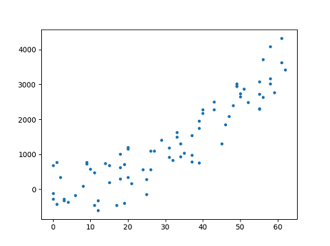
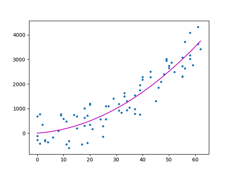
Many times the data we have, cannot be fitted linearly and we need a higher degree polynomial ( like quadratic or cubic ) to fit the data. We can use a polynomial model when the relationship between outcome and explanatory variables is curvilinear as can be seen in the given figure.

This article requires the understanding of linear regression and the mathematics behind it. If you are not aware about it then you can refer to my previous article on Linear Regression.

Introduction

Polynomial regression is a form of regression analysis in which the relationship between the independent variable x and the dependent variable y is modelled as an nth degree polynomial in x. However there can be two or more independent variables or features also.

Although polynomial regression is technically a special case of multiple linear regression, the interpretation of a fitted polynomial regression model requires a somewhat different perspective. It is often difficult to interpret the individual coefficients in a polynomial regression fit, since the underlying monomials can be highly correlated. For example, x and x² have correlation around 0.97 when x is uniformly distributed on the interval (0, 1).

Linear Algebra Review

Rank of a matrix

Suppose we are given a mxn matrix A with its columns to be [ a₁, a₂, a₃ ……a_n ]. The column a_i is called linearly dependent if we can write it as a linear combination of other columns i.e. a_i = w₁a₁ + w₂a₂ + ……. + w_i-1a_i-1 + w_i+1a_i+1 +….. + w_na_n where at least one w_i is non-zero. Then we define the rank of the matrix as the number of independent columns in that matrix. Rank(A) = number of independent columns in A

However there is another interesting property that the number of linearly independent columns is equal to the number of independent rows in a matrix.(proof)

Hence Rank(A) ≤ min(m, n) A matrix is called full rank if Rank(A) = min(m, n) and is called rank deficient if Rank(A) < min(m, n).

Pseudo-Inverse of a matrix

A nxn square matrix A has an inverse A^-1 if and only if A is a full rank matrix. However a rectangular mxn matrix A does not have an inverse. If A^T denotes the transpose of matrix A then A^TA is a square matrix and Rank of (A^TA) = Rank (A) (proof).

Therefore if A is a full-rank matrix then the inverse of A^TA exists. And (A^TA)^-1A^T is called the pseudo-inverse of A. We’ll see soon why it is called so.

Polynomial Fitting

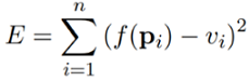
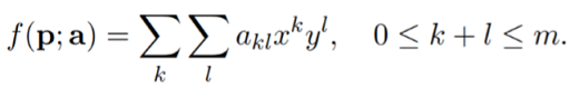
In general, non-linear fitting is more difficult than linear fitting. However we will be using a simple version. In Polynomial regression, the original features are converted into Polynomial features of required degree (2,3,..,n) and then modeled using a linear model. Suppose we are given n data points p_i = [ x_i1 ,x_i2 ,……, x_im ]^T , 1 ≤ i ≤ n , and their corresponding values v_i . Here m denotes the number of features that we are using in our polynomial model. Our goal is to find a nonlinear function f that minimizes the error Hence f is nonlinear over p_i .

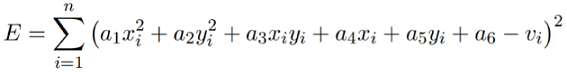
So let’s take an example of a quadratic function i.e. with n data points and 2 features. Then the function would be

The objective is to learn the coefficients. Hence we have n points p_i and their corresponding values v_i ; we have to minimize

For each data point we can write equations as

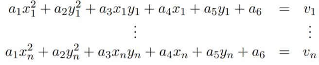
Hence we can form the following matrix equation

Da = v

where

However the equation is nonlinear with respect to the data points p_i , it is linear with respect to the coefficients a. So, we can solve for a using the linear least square method.

We have

Da = v

multiply D^T on both sides

D^TDa = D^Tv

Suppose D has a full rank, that is when the columns in D are linearly independent, then D^TD has an inverse.Therefore

(D^TD)^-1(D^TD)a = (D^TD)^-1D^Tv

We now have

a = (D^TD)^-1D^Tv

Comparing it with Da = v, we can see that (D^TD)^-1D^T acts like the inverse of D. So it is called the pseudo-inverse of D.

The above used quadratic polynomial function can be generalised to a polynomial function of order or degree m.

Underfitting and Overfitting

Underfitting and Overfitting are the most common problems in a machine learning model and lead to poor performance.

Underfitting refers to a condition when a model does not learn the features of training data and also cannot perform good on unseen data. Like if we want to fit a line in data with curvilinear pattern then the model will definitely underfit and cannot be used.

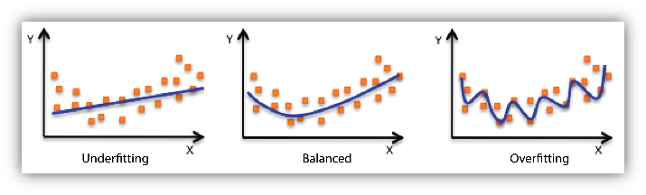
Overfitting refers to a condition when a model learns the data and the noise present in it so well, that it declines the performance of the model on the unseen data. Using a higher degree polynomial, say of degree 4 or 5, then it surely fit the training data very well but will produce high error for unseen data. Then the model will be overfit and again cannot be used.

Bias-Variance Tradeoff

Bias is how far are the predicted values from the actual values. If there is so much difference in the predicted values and the actual values then we say the bias is high.

Variance tells us how scattered are the predicted values from the actual values. High variance causes overfitting which means that our model is learning the noise present in the data.

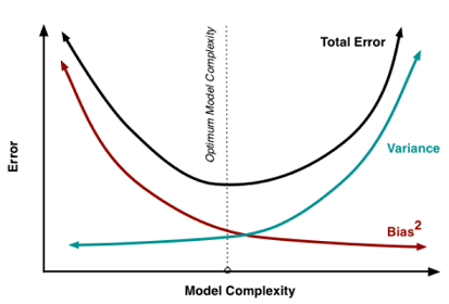
Bias-Variance Tradeoff

This figure depicts the bias-variance tradeoff in a very good way. It can be seen that as the complexity of the model increases i.e. if we use so many features or use a higher degree polynomial model to fit the data then the variance increases and bias decreases.

I hope now that you are clear with the working of polynomial regression and the mathematics behind. Next step will be to implement a polynomial model on a dataset using scikit-learn library. So get started.

Thanks for reading :)